

 Dr. Mathew Davies
Connecting Posit Workbench (RStudio) to GitHub with HTTPS
If you're an RStudio user using Posit Workbench and want to use GitHub for source control (you should), this is the guide for you. There are two ways...

Selecting a poor analytical modelling technique undermines a project before it starts. Choosing a good technique that’s wrong for the problem is as bad. It’s important to understand which techniques perform well in particular circumstances.
Here’s a true but cautionary tale about a technique that analysts use to perform minor miracles in certain domains failing to perform in another. The technique is Saaty’s Analytical Hierarchy Process (AHP). The problem is predicting football results.
Read on to learn a bit about Saaty’s AHP, see the technique used for predicting football results and watch an analyst losing money.
The problem isn’t Saaty’s technique. It’s just that some things are plain difficult to predict: for example human behaviour, tomorrow’s weather, and the outcomes of football matches.
But just because modelling these things is difficult doesn’t mean that we shouldn’t have a go.
I’m going to focus on that final problem. If it was easy to predict the outcomes of football matches, all analysts would be millionaires, right? They aren’t. There’s a reason for that.
Short and techy answer: Saaty’s AHP employs “pair-wise comparisons” to rank “options” against a set of “assessment criteria”.
More informative answer: Saaty’s AHP is the Swiss army knife of decision-making. It’s small, it’s (relatively) simple and you can apply it to a huge range of problems, from ranking the importance of different prisons, through selecting an outsourcing partner, to major procurement decisions.
Imagine you’re deciding where to go on holiday. The “options” are Spain, France, Belgium or Greece. Let’s suppose that the things you consider important in a holiday are: (1) the total costs of travel and accommodation; (2) the quality of the hotel; (3) the climate at your destination; and (4) the scope for entertaining yourself while away. You judge and compare the options against these “assessment criteria”.
You start the Saaty process by comparing pairs of assessment criteria against each other, asking: (a) which of these is more important to me; and (b) by how much is one of these criteria more important than the other. Saaty provides a standard set of phrases for describing the importance of one assessment criterion relative to another:
The numbers on the right-hand side provide a numerical coding for these judgements. As an example of the system’s use, suppose that you consider the climate to be strongly more important than entertainment; you would describe this situation by saying that the “weight” you afford to the climate is five (5) times greater than the weight you ascribe to entertainment. You store the resulting set of (weight ratio) numbers in a matrix and use a natty piece of maths to convert the full set of pair-wise comparisons into a corresponding weight for each of the assessment criteria.
Next up, you pick one of the assessment criteria, say total costs, and then compare all pairs of options against one another, asking the questions: (a) which of these options do I consider better in terms of total costs; and (b) by how much is one of these options better than the other for total costs? The answers to these questions are once again coded up using a system entirely analogous to that used previously when comparing assessment criteria; they are placed in a matrix; the natty bit of maths is brought out; and each of the options emerges from the process with a “score” against the assessment criterion under consideration; that’s the total cost in our example here. This process is repeated for each of the assessment criteria.
At this point, we have a score for each of the options against each of the assessment criteria. For example, perhaps the option to holiday in Spain scores 0.6 for total cost, 0.5 for the quality of the hotel, 0.7 for the weather and 0.3 for entertainment. At the same time, perhaps we give a weight of 0.9 to the total cost, 0.3 to the quality of the hotel, 0.7 to the weather and 0.5 to entertainment. We can then calculate a final, weighted score for Spain by multiplying the score for each assessment criterion against its associated weight and adding the results together:
(0.6*0.9) + (0.5*0.3) + (0.7*0.7) + (0.3*0.5) = 1.33
After repeating for each of the other options, we can finally rank our holiday options and so select the best.
Bear with me.
My mum was always scathing about get-rich-quick books. Why? Because:
Mum had a point.
It’s similar with anyone who tells you they know how to make money from betting on the results of football matches. I have tried to do this (and failed miserably) using Saaty’s AHP. Why Saaty’s AHP? Well, I have used it quite a bit in my day job for making decisions and what is the prediction of football results other than decision-making?
First, let’s assume that it makes sense to talk about a single number that sums up just how good each football team is. Let’s assume that this “goodness” figure lies somewhere between zero (0) and one (1): a team with zero “goodness” will likely be beaten by every other team and end up towards the bottom of their league. At the other extreme, a team with unit “goodness” is unlikely to be beaten by others and so is inclined to end up towards the top of their league.
Second, let’s assume that when two football teams play one another, the team with the higher “goodness” is more likely to win than its opponent; as a slight extension of this idea, a match between teams with similar “goodness” factors is more likely to result in a draw.
Third, we assume that the difference in numbers of goals scored by the teams competing in a football match is a reliable reflection of the difference in “goodness” factors between the two teams. As an embellishment of this idea, let’s assume that our best estimate of the ratio between the “goodness” factors of two teams after they have completed a match in which the winning team scores A goals and losing team scores B goals is two raised to the power of the goal difference, i.e. 2^(A-B) in favour of the winner. So a final score of Rovers 3-2 United means that the “goodness” factor for Rovers is roughly twice [2^(3-2)=2^1=2] the “goodness” factor of United. We would have arrived at the same conclusion had the score ended at 2-1 or 1-0 in Rovers’ favour
Now we can stop here and argue about the approach and assumptions described above, or we can press on. I’m going to argue for pressing on.
I’m going to suggest that we treat all teams as being identical at the very start of a new season. If there are N teams in the league, let’s say that we assume the “goodness” of each to be 1/N. I could have chosen to assume all teams as having a “goodness” of one-half, or exactly one, or something else and the answers would have been the same but I quite like the idea of normalising the goodness factors so that they sum to one when aggregated up across all teams in the league.
On completion of all matches on the first weekend of the season, we have N/2 results. Each of those results provides an estimate of how much better each winning team is than their defeated opponent; or, in the case of draws, confirmation that the teams are of roughly equal “goodness”. I’ll store that information in a matrix. Figure 1 shows an example of this so-called Pairwise comparison matrix (PCM) for the German Bundesliga, the only league in operation at the time of writing this blog, on the opening day of the season.
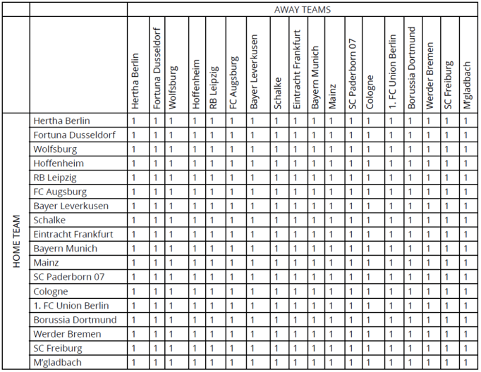
The entry at the intersection of the row specifying a particular home team and the column representing a particular away team contains the ratio of the home team’s “goodness” factor to the away team’s “goodness” factor. In Figure 1, I have assumed that all teams have the same “goodness” prior to the first match of the season and so all cells contain a ratio of 1.
As the season progresses and fixtures are played, so the PCM cells corresponding to those games are populated with the ratio of “goodness” factors for the teams involved, using our 2^(A-B) formula. Figure 2 shows the situation on Tuesday, 26th May 2020, shortly after the Bundesliga resumed games during the COVID-19 outbreak.
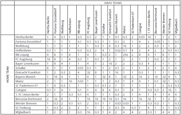
The value of 256 at the intersection of the RB Leipzig row and the Mainz column results from the match on Saturday, 2nd November 2019 in which the final score was RB Leipzig 8-0 Mainz. Hence, on that date, RB Leipzig was deemed to have a “goodness” factor some 2^(8-0) = 2^8 = 256 times better than that of their opponents, Mainz.
As you can imagine, the contents of this table (or PCM) reveal all sorts of inconsistencies between the performances of teams. Only some of this inconsistency can be removed by “averaging” over the results obtained when the same pair of teams played one another at each of their grounds. We are going to ignore such subtleties here and simply press on.
Given the PCM at a particular point in time, we can generate an estimate for the absolute “goodness” of each team on that same date. This is based on the mathematical technique of finding the eigenvector corresponding to the largest eigenvector of the PCM. In the case of the PCM shown in Figure 2, the corresponding results were as follows.
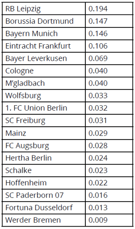
Based on our “goodness” estimates, RB Leipzig were ranked as the top team in the Bundesliga at that time, whereas Werder Bremen were ranked lowest. Moreover, by taking the ratio of “goodness” factors for all pairs of teams due to play each other over the following days, it was possible to generate the following predictions of match outcomes.
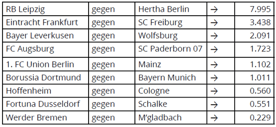
The most likely home victory was predicted for RB Leipzig (where the ratio was >> 1); the most likely away win was predicted for Munchen Gladbach’s fixture away to Werder Bremen (where the ratio was << 1); while the Borussia Dortmund game against Bayern Munich (with a ratio of around 1) looked most likely to end up as a draw.
In fact, the scores of these games turned out to be radically different, as shown below….
RB Leipzig 2 – 2 Hertha Berlin
Eintracht Frankfurt 3 – 3 SC Freiburg
Bayer Leverkusen 1 – 4 Wolfsburg
FC Augsburg 0 – 0 SC Paderborn 07
1. FC Union Berlin 1 – 1 Mainz
Borussia Dortmund 0 – 1 Bayern Munich
Hoffenheim 3 – 1 Cologne
Fortuna Dusseldorf 2 – 1 Schalke
Werder Bremen 0 – 0 M’gladbach
With the arguable exception of the FC Augsburg versus SC Paderborn 07 game, all my predictions were wrong. As I can testify to my expense, randomly selecting the results of the game would have been more likely to win money. That’s just one of the reasons why analysts are not millionaires.
It’s certainly not that there’s something wrong with Saaty’s AHP; as I know from experience, within the appropriate domain it produces very impressive results. The critical thing is knowing when and where it’s sensible to deploy the technique.
The problems with predicting football results arise from a combination of factors; not least, the high level of risk and intrinsic uncertainty in the outcome of matches, combined with an overly simplistic model of a team’s performance.
The key takeaways here for any budding mathematician/gambler are:
1. A football match is a surprisingly complex system (unfortunately)
2. Applying too simple a model to a complicated system will often end in tears (and empty wallets)
3. Even a reliable technique, like Saaty’s AHP, cannot save the day if undermined with an inadequate model
Anyone fancy a flutter?

If you're an RStudio user using Posit Workbench and want to use GitHub for source control (you should), this is the guide for you. There are two ways...

Many companies investing in data analytics struggle to achieve the full value of their investment, perhaps even becoming disillusioned. To understand...

We are cursed to live in interesting times. As I write this, a war in Ukraine rumbles on, we sit on the tail of a pandemic and at the jaws of a...